Template:Table/Template:InheritValueTable: Difference between revisions
| [unchecked revision] | [checked revision] |
No edit summary |
(railML→{{rml}}) |
||
| (23 intermediate revisions by 2 users not shown) | |||
| Line 1: | Line 1: | ||
{{ | <noinclude>{{tableDocu}} | ||
</noinclude> | |||
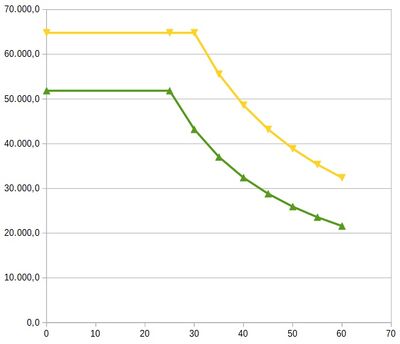
This is an example for usage of {{RS:Tag|valueTable}} with a series of two curves (force vs. speed) which are differentiated by a constant power limitation. | |||
{| | |||
|[[File:Force-diagram.jpg|400px]] | |||
|style="width:100px"| | |||
| | |||
{| | |||
!Speed | |||
!Force100 | |||
!Force66.7 | |||
|- | |||
|0 | |||
|64.800,9 | |||
|51.840,0 | |||
|- | |||
|25 | |||
|64.800,9 | |||
|51.840,0 | |||
|- | |||
|30 | |||
|64.800,9 | |||
|43.200,0 | |||
|- | |||
|35 | |||
|55.542,9 | |||
|37.028,6 | |||
|- | |||
|40 | |||
|48.600,0 | |||
|32.400,0 | |||
|- | |||
|45 | |||
|43.200,0 | |||
|28.800,0 | |||
|- | |||
|50 | |||
|38.880,0 | |||
|25.920,0 | |||
|- | |||
|55 | |||
|35.345,5 | |||
|23.563,6 | |||
|- | |||
|60 | |||
|32.400,0 | |||
|21.600,0 | |||
|} | |||
|- | |||
|Graphical representation of the curves. | |||
| | |||
|The value table in a spreadsheet. | |||
|} | |||
;{{rml}}-Code: | |||
<syntaxhighlight lang=xml> | |||
=== | <valueTable yValueUnit="N" xValueName="speed" yValueName="tractive effort" | ||
xValueUnit="km/h" zValueName="Percentage power limitation" zValueUnit="%"> | |||
<columnHeader zValue="100" /><columnHeader zValue="66.7" /> | |||
<valueLine xValue="0.0"> | |||
<values yValue="64800" /><values yValue="51840" /> | |||
</valueLine> | |||
<valueLine xValue="25.0"> | |||
<values yValue="64800" /><values yValue="51840" /> | |||
</valueLine> | |||
<valueLine xValue="30.0"> | |||
<values yValue="64800" /><values yValue="43200" /> | |||
</valueLine> | |||
<valueLine xValue="35.0"> | |||
<values yValue="55542.9" /><values yValue="37028.6" /> | |||
</valueLine> | |||
<valueLine xValue="40.0"> | |||
<values yValue="48600" /><values yValue="32400" /> | |||
</valueLine> | |||
<valueLine xValue="45.0"> | |||
<values yValue="43200" /><values yValue="28800" /> | |||
</valueLine> | |||
<valueLine xValue="50.0"> | |||
<values yValue="38880" /><values yValue="25920" /> | |||
</valueLine> | |||
<valueLine xValue="55.0"> | |||
<values yValue="35345.5" /><values yValue="23563.6" /> | |||
</valueLine> | |||
<valueLine xValue="60.0"> | |||
<values yValue="32400" /><values yValue="21600" /> | |||
</valueLine> | |||
</valueTable> | |||
</syntaxhighlight> | |||
When using the {{RS:Tag|valueTable}} as representation of a series of curves (three-dimensional function) it shall be written in {{rml}} similar as in a spreadsheet. It means first the header has to be defined with the value descriptions. Second the particular z-values valid for each curve out of the series are to be listed as child element {{RS:Tag|columnHeader}}. Finally the respective {{RS:Tag|valueLine}} for each x-value of the curves is included. Per each x-value there must be as much y-values as the number of curves (number of z-values). The order of y-values is according the order of z-values. Thus a clear assignment to the related curve is made. It shall be noted that the x-values may be not equidistant. In case the original series of curves have different x-values then interpolation must be used to get the missing y-values per each x-value occurring in the series. | |||
Latest revision as of 22:24, 22 January 2024
This template contains swapped content from page Template:InheritValueTable
This is an example for usage of <valueTable> with a series of two curves (force vs. speed) which are differentiated by a constant power limitation.
- railML®-Code
<valueTable yValueUnit="N" xValueName="speed" yValueName="tractive effort"
	xValueUnit="km/h" zValueName="Percentage power limitation" zValueUnit="%">
	<columnHeader zValue="100" /><columnHeader zValue="66.7" />
	<valueLine xValue="0.0">
		<values yValue="64800" /><values yValue="51840" />
	</valueLine>
	<valueLine xValue="25.0">
		<values yValue="64800" /><values yValue="51840" />
	</valueLine>
	<valueLine xValue="30.0">
		<values yValue="64800" /><values yValue="43200" />
	</valueLine>
	<valueLine xValue="35.0">
		<values yValue="55542.9" /><values yValue="37028.6" />
	</valueLine>
	<valueLine xValue="40.0">
		<values yValue="48600" /><values yValue="32400" />
	</valueLine>
	<valueLine xValue="45.0">
		<values yValue="43200" /><values yValue="28800" />
	</valueLine>
	<valueLine xValue="50.0">
		<values yValue="38880" /><values yValue="25920" />
	</valueLine>
	<valueLine xValue="55.0">
		<values yValue="35345.5" /><values yValue="23563.6" />
	</valueLine>
	<valueLine xValue="60.0">
		<values yValue="32400" /><values yValue="21600" />
	</valueLine>
</valueTable>
When using the <valueTable> as representation of a series of curves (three-dimensional function) it shall be written in railML® similar as in a spreadsheet. It means first the header has to be defined with the value descriptions. Second the particular z-values valid for each curve out of the series are to be listed as child element <columnHeader>. Finally the respective <valueLine> for each x-value of the curves is included. Per each x-value there must be as much y-values as the number of curves (number of z-values). The order of y-values is according the order of z-values. Thus a clear assignment to the related curve is made. It shall be noted that the x-values may be not equidistant. In case the original series of curves have different x-values then interpolation must be used to get the missing y-values per each x-value occurring in the series.
